Let us start with a brief recap of the biology of gene expression. A genome is a string of nucleotides A, C, G and T. This string is the source code for proteins that the cell can produce. Proteins are strings of amino-acids, where the amino-acids are selected from a set of 20 naturally occurring types. A string of nucleotides A, C, G and T is translated into a string of amino acids by interpreting consecutive non-overlapping triplets (3-mers) of nucleotides as codewords (codons) for the different kinds of amino acids. Since the number of possible distinct triples of nucleotides is 64, and there are only 20 distinct amino acids, most amino acids are encoded by multiple different codons. Two codons that encode the same amino-acid are called synonymous.
It is known that bacterial species tend to favor some synonymous DNA codons over others. This phenomenon is called codon bias. The reason for these biases is a debated topic in molecular evolution. One explanation is that differences in the transfer RNA (tRNA) pool of the cell lead to discrepancies in the transcription efficiency of synonymous codons, which leads to mutational pressure toward the more efficient codons.
It turns out that every species has a unique characteristic codon bias. This suggests that the molecular pathway from DNA to protein favors different codons in different bacteria. It is not clear whether codon bias evolves to adapt to the tRNA pool and other conditions in the cell, or vice versa.
In this post we examine the codon usage and k-mer statistics of a reference genomes of Escherichia coli and Vibrio cholerae.
3-mer distributions
First, let’s just plot the distribution of nucleotide triplets in E. coli.
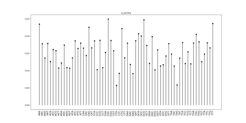
There is a pattern in this distribution: the frequency of a 3-mer is strongly correlated with frequency of its reverse complement. This can be seen clearly when we scatterplot the frequencies of a 3-mer against the frequency of the reverse complement.
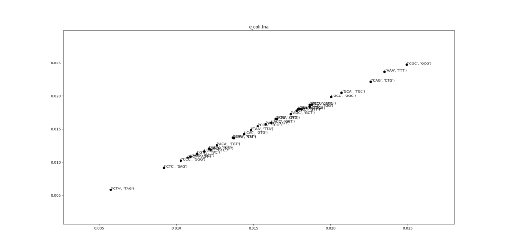
This can be explained by the double stranded structure of DNA. Genes are encoded in both complementary strands of the DNA, and one strand is the reverse complement of the other. The reference genome is just one arbitrarily chosen strand of the DNA, and genes from the other strand appear reversed and complemented on the reference strand. The same selective pressures for codons apply in the reverse complement.
Let us now check the codon distribution of V. cholerae:
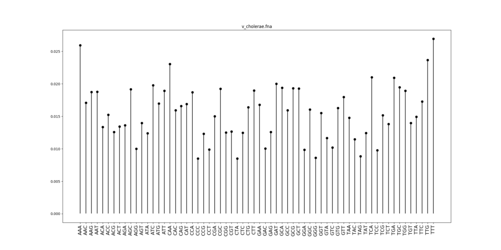
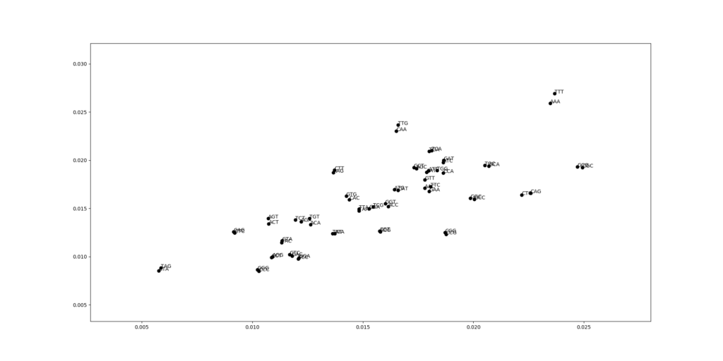
These statistics are quite different compared to E. coli. To see better, let us draw the scatterplot comparing codon frequencies between E. coli and V. cholerae. Each dot is one codon, the x-coordinate gives the frequency in E. coli, and the y-coordinate the frequency in V. cholerae.
Barcodes
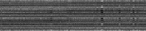
It also turns out that the codon usage statistics remain stable over the whole genome. To visualize this, we use the barcode plot, introduced by Fengfeng Zhou, Victor Olman and Ying Xu. In the method, the genome is divided into non-overlapping segments (“windows”), and the 3-mer distribution of each segment is computed. The data is plotted as a black-and-white image, where each column represents a genome segment, each row represents a 3-mer, and the brightness of a pixel is proportional to the frequency of that 3-mer in that segment.
If the 3-mer composition remains the same in every segment, every row of pixels should have a constant brightness. Running the experiment confirms that this is approximately true. Below is the barcode plot of E. coli with a window size of 10000 nucleotides.

It’s a bit hard to see because the image is only 64 pixels tall, but it’s evident that there are long horizontal lines. However, there are some breaks in the lines. Perhaps those regions are recently acquired genes which have not yet been adapted to the codon usage patterns of the new host? In Vibrio cholerae, we see a longer horizontal break:
Building the barcode plot for quartets of nucleotides instead of triplets shows a similar pattern. Now each row represents a 4-mer and there are 4^4 = 256 rows.
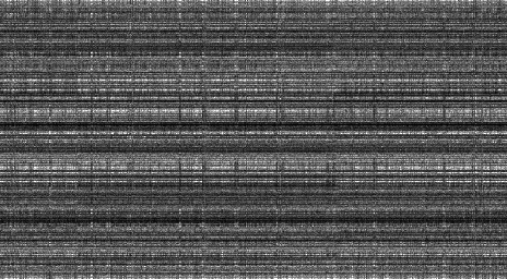

Decreasing the window size from 10000 to 1000 shows even more detail. Be sure to click the images for full-sized versions.

